Generative Adversial Networks (GAN) - Part 1

Generative Adversial Algorithm (GAN): Basics

This blog post was created from my personal notes of the specialisation course about GAN’s on coursera.org.

GANs are an emergent class of deep learning algorithms that generate incredibly realistic images. In this blog post I try to provide a look under the hood and to explain how GAN’s work and why they are useful.

There are many applications for GAN’s. For example, they can be used for the following tasks:

• Generate pictures, e.g. from people or artwork
• Modify images, e.g. make a person look older or younger
• Supervised learning tasks: Classify scratched objects or generate additional images
• many more …

I will address some of these use cases in this blog post. But first, I would like to give an overview about GAN’s and roughly describe how they work. Later, I will explain the network in more detail and provide some examples.

Intuition about GAN’s

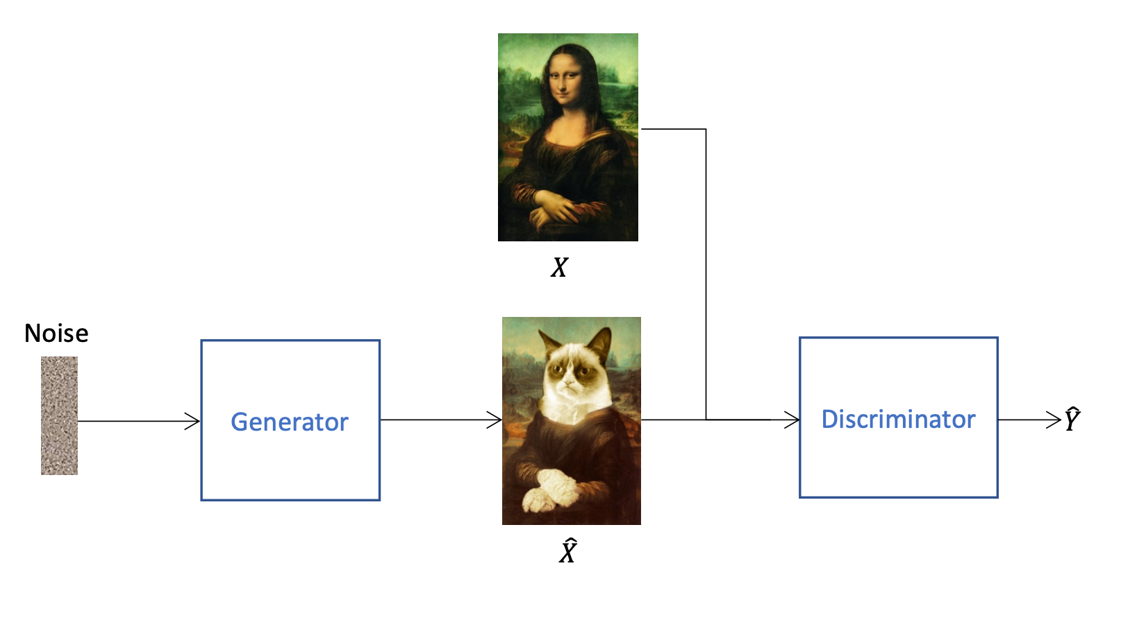
GAN’s are a unsupervised learning technique. Behind a GAN are two different models: The generator and the discriminator. The generator generates data, wheras the discriminator evaluates the generated data. To make the explanation less abstract, we will assume in this blog post that the generator creates images and the discriminator validates them (although GAN’s can be used for other data than images).

After the generator has created an image \(\hat{X}\), the discriminator tries to find out whether an image is real or has been generated (output \(\hat{Y}\)). To ensure that the discriminator cannot label all images as generated, not only generated but also real images \(X\) are fed in. That cyclic process is a zero-sum game between thse two models, which means the models “fight” against each other. The generator generates an image, afterwards the discriminator validates if it is generated ot not. Once the generator has learned to create more realistic images, the discriminator learns to recognise the fakes even better. This process is repeated continuously and both models eventually become better. For this to work, we must not only fed the images from the generator to the discriminator, but also real images. Otherwise the discriminator could label all images as fake and would then always be right. In the end, we no longer need the discriminator and only use the generator to create new images.

To prevent the generator from always producing the same images, a noise vector is used as input. This is a vector which is generated randomly and effects the output accordingly.

The generator and the discriminator are both neural networks that need to be trained. It is very important that both networks are trained at the same time and always have about the same skill level. The discriminator has an easier task to learn, because it only has to determine whether an image is real or not. The generator, on the other hand, has to create much more complex features. If the discriminator is much better than the generator, the problem arises that it can tell with almost 100% certainty whether a picture is real or fake. In this case the generator cannot learn because it cannot determine if its adjustments lead to a better result if the feedback from the discriminator is always 100% fake.

How the Discriminator learns

To improve the prediction of the discriminator, the parameters \(\theta_D\) must be updated. For this purpose, generated and real images are fed into the discriminator. Afterwards the discriminator makes a prediction between \([0...1]\), if the image was a generated or not. Based on this prediction \(\hat{Y}\) and the groundtruth \(Y\) (what was really fed into the discriminator) the BCE-loss is calculated and by backpropagation the parameters are updated accordingly.

How the Generator learns

Compared to the discriminator, the generator needs a different architecture to learn. If the generator is trained, then no real images are fed into the discriminator, because in this case only the BCE-loss for the generated images is of interest.

So the discriminator makes a prediction for generated images each time. The worse the prediction of the discriminator is, the better the generator becomes. It is important that only the parameters of the generator are updated and not the discriminator. Otherwise the discriminator would update the parameters incorrectly if it does not receive real images in between.

BCE Cost Function

The Binary Cross Entropy cost function is one the simplest functions to train GAN’s. The function is defined as:

where

• \(m\) is the batch size and \(x^{(i)}, y^{(i)}\) are the features and labels from a specific example
• \(\theta\) are the parameters to update
• \(h(x,\theta)\) is a function which predicts the label for a given set of features \(x\) and some parameters \(\theta\)

The first part of the equation \(\frac{1}{m} \sum^m_{i=1}\) just means that we average over the whole batch. The term inside the rectangular brackets can be broken down into two parts:

1. \[y^{(i)} \log h(x^{(i)}, \theta)\]
2. \[(1-y^{(i)}) \log (1-h(x^{(i)}, \theta))\]

To become some intuition about this term, let’s look at the first part. The label is multiplied with the log of the prediction: \(y^{(i)} \log h(x^{(i)}, \theta)\). If the label \(y^{(i)}\) is zero (e.g. means image is fake), then the whole term becomes \(0\). If the label \(y^{(i)}\) is one and the prediction \(h(x^{(i)}, \theta)\) is one, the term also becomes zero. But if the label \(y^{(i)}\) is one and the prediction \(h(x^{(i)}, \theta)\) is almost 1, the term becomes very large. That means that this first term is the loss for one example if the label \(y^{(i)}\) is one. The loss becomes larger in a logarithmic ratio if the prediction is inaccurate (value is less than 1). The second term does the same for the case where the label \(y^{(i)}\) is 0.

Improving the GAN’s

With BCE loss GANs are prone to mode collapse and vanishing gradient problems. A mode collapse means that the generator no longer generates all modes from the data distribution. To understand this, imagine the following example: The generator should generate the letters “A”, “B”, “C”, “D”, and “E”. But the discriminator is already relatively good and recognizes the generated letters “A”, “C” and “D” with high confidence as fake. This has the consequence that the discriminator returns a value \(~ \approx 1\) (fake) for these letters. Since the activation function is a sigmoid function, the derivative of this is almost \(\approx 0\) and the generator cannot learn. This then has the consequence that the generator no longer produces the letters “A”, “C” and “D”. This is so called a mode collapse: Instead of generating all five letters the generator only generates the two letters “B” and “D”.

So the problem with BCE loss is that as a discriminator improves, it returns values closer to zero and one. But this return values are not really helpfull for the generator to further improve. As a result, the generator stops learning due to vanishing gradient problems. To overcome these problems, a good idea is to calculate the distance between the real and the generated images. Therefore, often the Earth Movers Distance is used.

With Earth mover’s distance, there’s no such ceiling to the zero and one as with the BCE-Loss. This is because the eath movers distance measures how different two distributions are based on distance and amount. The output of this function must not be between 0 and 1 but is just a real number. Therefore, we can use this measurement to calculate the distance between the real and generated images. As a result, we won’t get a number between 0 and 1 as with the BCE loss, but a distance. That means that the cost function continues to grow regardless of how far apart these distributions are. The gradient of this measure won’t approach zero and as a result, GANs are less prone to vanishing gradient problems and from mode collapse.

The Wasserstein loss is a loss function which approximates the Earth Mover Distance. It looks pretty similar than the BCE loss but has nicer properties. Because the Wasserstein loss returns a distance and no value between 0 and 1 and therefore does not discriminate between classes the discriminator is usually called Critic. The Wasserstein loss measures the distance between the output of the Critic \(c\) of a real image \(x\) and a generated image \(g(x)\). This is dennoted as:

The goal of the citric is to maximize this distance, whereas the generator tries to minimize the distance. In order for the Wasserstein loss to work well, it must fullfill the 1-Lipschitz continous condition. This condition says that the norm of the gradients of the critic output should be at most 1 at every output. That just means that the output function can max. Increase or decrease lineally. Otherwise the loss would grow to much and there would not be enough stability during training. The 1-L continous condition is fulfilled if:

This condition can be enforced during training with weight clipping. Weight clipping means that we calculate the weight update with gradient descent and if the weight change is outside the allowed limit, we just set the weights to the maximum allowed value. The disadvantage of this method is that forcing the weights of the critic to a limited range of values could limit the critics ability to learn. Therefore, it is recommended to use a gradient penalty instead of weight clipping. With gradient penalty we just add a regularization term \(r\) to the loss function. This term penalizes the critic when it’s gradient norm is higher than one.

But it is not practical to check the critic’s gradient at every possible point. Instead we sample just some points by interpolating between real and fake examples. We call these interpolated images \(\hat{x}\). The goal is that the gradient of this \(\hat{x}\) is one. Therefore, we improve the Wasserstein loss function as follows:

Implementation in Python using PyTorch

Get the gradient from a real and a fake image:

def get_gradient(crit, real, fake, epsilon):
    '''
    Return the gradient of the critic's scores with respect to mixes of real and fake images.
    '''
    # Mix the images together
    mixed_images = real * epsilon + fake * (1 - epsilon)

    # Calculate the critic's scores on the mixed images
    mixed_scores = crit(mixed_images)
    
    # Take the gradient of the scores with respect to the images
    gradient = torch.autograd.grad(
        inputs=mixed_images,
        outputs=mixed_scores,
        grad_outputs=torch.ones_like(mixed_scores), 
        create_graph=True,
        retain_graph=True,
    )[0]
    return gradient

calculate the gradient penalty:

def gradient_penalty(gradient):
    '''
    Return the gradient penalty, given a gradient.
    Given a batch of image gradients, you calculate the magnitude of each image's gradient
    and penalize the mean quadratic distance of each magnitude to 1.
    '''
    gradient = gradient.view(len(gradient), -1)
    gradient_norm = gradient.norm(2, dim=1)
    penalty = torch.mean((gradient_norm - 1)**2)
    return penalty

Calculate the loss of the generator and the critic:

def get_gen_loss(crit_fake_pred):
    '''
    Return the loss of a generator given the critic's scores of the generator's fake images.
    '''
    gen_loss = -torch.mean(crit_fake_pred)
    return gen_loss
  
 def get_crit_loss(crit_fake_pred, crit_real_pred, gp, c_lambda):
    '''
    Return the loss of a critic given the critic's scores for fake and real images,
    the gradient penalty, and gradient penalty weight.
    '''
    crit_loss = torch.mean(crit_fake_pred) - torch.mean(crit_real_pred) + c_lambda * gp
    return crit_loss

Conditional Generation

With unconditional generation are just outputs from a different class generated. If again the letters “A”, “B”, “C”, “D” and “E” are to be generated, we cannot control for example which letter the generator generates. With condotional generation we can train an network to generate a specific class, for example the letter “E”.

With conditional generation we do not only need a noise vector to feed into the generator network, but also a class vector (one-hot vector). This class vector specifies which class the generator should generate. Instead of feeding two individual vectors into the network, we attach the noise vector and the class vector together.

However, the class vector must not only be fed into the generator but also into the discriminator (the critic). The discriminator will not only give a low value (\(\approx 0\)) if it is a generated image, but also if the wrong class (e.g. the letter “A” instead of “E”) was generated. As with the generator, the class vector is not fed into the network individually but in this case as additional channels of the image.

For this to work, the network must of course know what the individual classes are. Therefore the data must be labelled. Using these labels the network can learn different classes during the training. After the training the class can be specified and the network generates a corresponding image.

Controllable Generation

Controllable generation allows to control some of the features that are in the output example. For instance, with a GAN that generates faces, we could control the age of the person’s looks or the gender. This can be done by tweaking the input noise vector, that is fed to the generator.

Compared to Conditional Generation, we do not generate different classes but tweak some individual features of the classes. Therefore the network does not need labels during the training. Furthermore, the individual features are tweaked after and not during the training.

Idea behind Controllable Generation: If we can create a letter “E” in block letters with a noise vector and the letter “E” in string writing with another noise vector, then we can interpolate linearly from the first noise vector to the second noise vector. So we can calculate the difference between these two vectors and add it to a noise vector which produces the letter “A” in block letters. The result is then the letter “A” in string writing.

To learn these vectors an additional classifier can be used. For example, a pre-trained string font classifier can be used. This classifier recognises whether a letter is written in block letters or in string writing. This classifier is only used to find the corresponding noise vector. So we feed different noise vectors into the generator, but the weights of the generator are not adjusted. The output of the generator is then fed into the additional classifier, which gives a feedback if the generated letter is written in string writing. This allows the features in the noise vector to be searched automatically.