Generative Adversial Networks (GAN) - Part 2

Generative Adversial Algorithm (GAN): Advanced

This blog post was created from my personal notes of the specialisation course about GAN’s on coursera.org.

In this second part about GAN’s I try to explain cutting edge algorithm to create much more realistic images and also how models can be evaulated. Additionally, I provide a short overview about alternatives to GAN’s such as the VHV model.

Evaluation of GAN’s

Evaluating GANs is a particularly challenging task, because we normally don’t have labels to evaluate if the result is correct or not like in supervised learning. Additionally, the discriminator often overfits the generator and even if the images from the generator looks realistic, the discriminator finds out that they are generated based on some very small almost invisible features in the image. Therefore, there does not exist an universal gold-standard discriminator.

To evaluate a GAN we can define different porperties such as:

• Fidelity (quality of the image)
• Diversity (variety of images)
• …

There are a lot of properties possible, but the both above are most commonly used. To measure the fidelity, we measure how different the image is from it’s nearest real image. To measure the diversity we compare the spread of a set of generated images with the spread of real images. It is often a tradeoff because these two properties, because fidelty measures the difference to real images and diversity the spread of the generated images compared to real images.

To compare two images we could measure the pixel distance, but this is often insufficient. Instead we compare the features of the images an measure their distance. For example if we have a real and a generated image of a cat we do not compare the pixels between these two images but features such as a “cat has two ears”, “mouth is below nose”, … . This measurement is much more reliable than the pixel distance.

To compare these features, they must first be extracted from the images. Therefore, often a pertained classifier is used as feature extractor. This classifiers are pre-trained on large datasets such as ImageNet. If the fully connected layers at the end are removed, we end up with a pretrained CNN. The last layer of this CNN provides pretty good features, which can then be used to extract the features from the images.

Fréchet Inception Distance (FID)

The most popular metric to measure the distance between features is the Fréchet Inception Distance. The Fréchet distance was originally used to calculate the distance between to curves, but can also be used to measure the distance between distributions. To Fréchet distance between two single dimensional, normal distribution is defined as

\[d(X,Y)=(\mu_X-\mu_Y)^2 + (\sigma_X-\sigma_Y)^2\]

where \(\mu_A\) is the is the mean of a distribution \(A\) and \(\sigma_A\) the standard deviation of \(A\). So it is just the difference between the mean and the standard deviation. This formula can be generalized to multvariant normal distributions. The multivariante normal Fréchet Distance is defined as

\[||\mu_X-\mu_Y||^2 + \text{Tr}(\textstyle \sum\nolimits_{X} + \textstyle \sum\nolimits_{Y} - 2 \sqrt{\textstyle \sum\nolimits_{X}\textstyle \sum\nolimits_{Y}})\]

where \(\textstyle \sum\nolimits_{A}\) is the covarinace matrix and \(\text{Tr}\) is the trace of a matrix (sum of diagonal elements). This multivariant distance is almost the same as the univariant distance. The first part

\[||\mu_X-\mu_Y||^2\]

is again the square of the distance between the centers, but since there are multiple distributions, the L2-Norm is used. The second part

\[\text{Tr}(\textstyle \sum\nolimits_{X} + \textstyle \sum\nolimits_{Y} - 2 \sqrt{\textstyle \sum\nolimits_{X}\textstyle \sum\nolimits_{Y})}\]

is again the squared difference of the standard deviation. If we multiply out the standard deviation distance in the univariant formula

\[(\sigma_X-\sigma_Y)^2 = (\sigma_X^2 + \sigma_Y^2 + 2\sigma_X\sigma_Y)\]

we see the relation to the multivariant version.

The real and the generated embeddings are two multivariante normal distribution. With the Fréchet Inception Distance we can calculate he distance between theese two distributions. The lower the distance is, the more similar are the features. Therefore, the goal is to minimize this distance. To reduce the noise it is recommended to use larger sample sizes.

GAN Improvements

Main improvements of GANs over the last years:

• Stability
  • Prevent mode collaps by measuring the standard deviation of the results
  • Ensure 1-Lipschitz continuity
  • Use multiple generator and use the averaged weight parameters
  • Use progressive growing: increase the image resolution over time
• Capacity
  • Larger model can use higher resolution images (larger model possible due to computational power)
• Diversity

A modern variant of GANs is called StyleGAN. StyleGAN is currently considered one of the best architectures and includes the above mentioned improvements. StyleGAN is described in more detail in the following chapter.

StyleGAN

StyleGAN can produce extremly realistic human faces. It provides increased control over image features such as hats or sunglasses and allows mixing styles from two different generated images together.

For example the following image is generated by a StyleGAN (refresh page to load a different image):

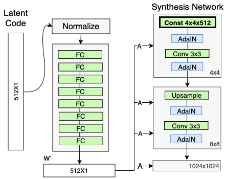
In a traditional GAN generator, the noise vector is directly fed into the generator and the generator then outputs an image. In StyleGAN, the noise vector is handled different. Instead of feeding in the noise vector directly into the generator, it goes through a mapping network to get an intermediate noise vector \(W\). This noise vector then gets injected multiple times into the StyleGAN generator, to produce an image. Additionally, there’s an extra random noise that’s passed in to add various stochastic variation onto this image.

The intermediate noise vector \(W\) is added to various layers in the StyleGAN generator. This injection of this intermediate noise into all of these layers of StyleGAN is done through an operation called AdaIN or adaptive instance normalization. AdaIN is like batch normalization, except that after normalisation, it tries to apply some kind of style based on the intermediate noise vector \(W\).

The 3rd and final important component of StyleGAN is progressive growing. This component slowly grows the image resolution being generated by the generator and evaluated by the discriminator over the process of training. So during the training process, both the generator and discriminator start with a small low resolution image.

This was only a brief overview of these components, which are described in more detail below.

Progressive Growing

Progressive growing is trying to make it so it’s easier for the generator to generate higher resolution images by gradually training it from lower resolution images to higher resolution images. To make it not so obvious for the discriminator what’s real or fake, the real images will also be downsampled on the same size than the generated images. Normally, the image size starts arround \(4\times4\) images and then by an upsampling task the size gets doubled.

The generator is normally a CNN with convolutional layers. The progressive growing isn’t as straightforward as just doubling the size of the last convolutional layer immediately at some scheduled intervals. In a first iteration the existing images are just upsampled. then in the next iteration for example \(99\%\) of the image are upsampled and \(1\%\) of the images is fed trough an new convolutional layer with the desierd new size. This is repeated several times until all the images are generated with the the new convolutional layer and no images are upsampled anymore.

For the discriminator there’s something fairly similar, but in the opposite direction. At the beginning, the images are downsampled. Then in the the next iteration \(99\%\) of the images are downsampled and \(1\%\) of the images is fed through an new convolutional layer. It is important, that the number of images which are fed through the conversation-layer is equal for the generator and the discriminator.

In summary, progressive growing gradually will double that image resolution so that it’s easier for the StyleGAN to learn higher resolution images over time. Essentially, this helps with faster and more stable training.

Noise Mapping Network

The noise mapping network takes the noise vector \(Z\) (which comes from a Gaussian distribution) and maps it into an intermediate noise vector \(W\). This noise mapping network is composed of eight fully connected layers with activations in between, also known as a multilayer perceptron or MLP. So it’s a pretty simple neural network that takes your \(Z\) noise vector, which is 512 in size and maps it onto the intermediate noise factor \(W\), which has the same size but changed values.

The motivation behind this is that mapping the noise vector will get a more disentangled representation. This allows a much more fine grained control about the features in the resulting image. For example adding some glasses does then not also end up with changing the hair color.

The intermediate noise vector \(W\) is then not fed in the first convolutional layer, but in all the different layers. The noise vector is added with the Adaptive Instance Normalization (AdaIN).

Adaptive Instance Normalization (AdaIN)

Adoptive Instance Normalization (AdaIN) is applied after each convolutional layer. First, the output of each convolution is normalized using Instance Noramalization. Therefore, the mean \(\mu(x)\) is subtracted from the output \(x\) and then this term is divided by the standard deviation \(\sigma(x)\):

\[\frac{x_i-\mu(x_i)}{\sigma(x_i)}\]

Compared to batch normalization, instance normalization looks at only one sample and not at the entire batch. The second step is then to apply adaptive styles using the intermediate noise vector \(W\). But \(W\) is not directly added to the normalized output. Instead \(W\) goes through two fully connected layers which then produces two parameters: The scale \(y_s\) and the bias \(y_b\). These parameters are then applied to the normalized output:

\[\text{AdaIN}(x_i,y)=y_{s,i}\frac{x_i-\mu(x_i)}{\sigma(x_i)}+y_{b,i}\]

Overview about the whole Achitecture

Other Architectures: Variational Autoencoders (VAEs)

There exists a lot of alternatives to GANs. A popular alternative are the variational auto encoders (VAEs). VAEs work with two different models: an encoder and a decoder. It learns by feeding real images into that encoder, finding a good way of representing that image in the latent space, and then reconstructing the realistic image the encoder saw before with the decoder. After training of the VAE we don’t need the encoder anymore and can just sample points from the latent space and then use the decoder to generate an output image.

The advantage of VAEs is that they have density estimation, a more stable training and are invertible. Invertible means, that we can feed in an image and then get the noise vector. After changing the noise vector a bit, we can produce the same image again but with small adjustments. For example, we could find the noise vector of a person, and then change the noise vector in order to make this person look older or to change the hair color. But the main disadvantage of VAEs is that they produce lower quality results.

Application of GAN

There are many different applications for GANs. Some are described in more detail in the following chapters.

Data Augmentation

Data augmentation is typically used to supplement data when real data is either too expensive to acquire or too rare. Typical data augmentation methods for images are:

• zoom in and crop the image
• apply different filters
• rotations or horizontal/vertical flips
• …

However, in the end it is still the same picture. A GAN, on the other hand, does not modify an existing image, but generates a large number of new images from the same class. These newly generated images usually have a much greater diversity than when only classical data augmentation methods are used. In addition, all other data augmentation methods can be applied to these generated images.

Pros:

• Improve downstream model generalization
• Often better than hand-crafted synthetic example
• Generate more labeled examples (especially useful for unbalanced or small classes)

Cons:

• Diversity is limited to the data available
• Can overfit to the real training data

GANs for Privacy and Anonymity

In some application such as in the medical field, privacy is very important. Often using real patient data in the models can harm the patients if someone reverse engineers the model and figures out who those people are or if that data is somehow released.

Besides privacy, GANs can also be used for anonymity. For example, the face from activists, witnesses ir victims can be replaced with another face and they would still be able to express themselfs in public. Then downside of this technology is that deep fake can be produced. For example a video could be created from a famous person where someone put some words in his mouth.

Image-to-Image Translation with Pix2Pix

Image translation is applying some transformation to an image in order to get a transformed version of it. For example adding colors to a black and white image or creating a realistic photo from a segmentation mask are typical translations.

The encoder of Pix2Pix takes instead of a noise vector and a one-hot encoded feature vector an entire image. This image could be a segmentation mask. In that case, Pix2Pix can then be trained to generate an image which corresponds to that segmentation mask. The discriminator then also gets this segmentation mask, together with the original mask from which the mask was derived or with the generated image. The discriminator then tries to find out if the image is the original or the generated one.