Self-Supervised Approaches

Ideas and Findings

Data set:

• State-of-the-art self-supervised approaches are mostly trained on Libri-Speech. This dataset contains approx. 960h of audio data.
• The TIMIT dataset is much smaller (approx. 6h) and could therefore be used for fine-tuning only
• A challenge will be the training time: E.g. wav2vec 2.0 used 128 V100 GPU's for pretraining and this setup still took more than 7 days.
  • It could be beneficial to look for a pretrained model

Input signal:

• Many state-of-the-art approaches uses the raw signal as input and then apply a CNN to extract representational features. They show that these feature vectors achieve better results on most downstream tasks than Mel-spectrograms or MFCCs. However, the goal of this project thesis is to predict speech. Therefore, it makes sense to use the same kind of signal as input and as output. The raw signal is considered as to noisy and therefore it is recommended to use Mel-spectrograms or MFCCs
  • Try to compress high-dimensional data into a much more compact latent embedding as done in CPC but do not remove necessary information for prediction (e.g. remove lokal noise but not more global noise)
• The Mel-spectrograms or MFCCs could still be fed into an CNN to extract more task specific features
• Use log Mel-spectrograms instead of Mel-spectrograms

Architecture:

• CNN pre-net to extract the needed features to predict future sequences
• RNN (GRU) model to predict the Mel-spectrogram or MFCC
• CNN post-net to smooth the predicted Mel-spectrogram or MFCC
• Should be fast in order to use a lot of data

Loss:

• Try L1 loss instead of L2 loss as done for speech synthesis
• Weight loss depending on the distance as done for continous skip-gram

Training ideas:

• Contrastive pretraining of the pre-net: Use a given sequence and the following sequence as positive example, use a given sequence and some random sequences as negative example
  • Does this preserve enough information to reconstruct signal?
• Train end-to-end as done at the moment but use other architecture and different loss
• Two steps: Instead of predicting directly Mel-spectrogram predict a simpler embedding which can reconstruct the spectrogram (combine CPC with some generic approach)
• Train an autoencoder first, then use the encoder to encode the given data and the target and learn to predict the encoded data, afterwards use the decoder to reconstruct the predicted encoded data

Models in natural language processing are pretrained in several different ways. For example, autoencoding models are pretrained by corrupting the input tokens and trying to reconstruct the original sentence. However, predicting the next frame of speech is closely related to autoregressive models in NLP: Autoregressive models are pretraind by guessing the next token having read all the previous ones. Although autoregressive models can be fine-tuned for many tasks, the most common application is text generation. State-of-the-art models like GPT v1-v3 or Transformer-XL use therefore the decoder of the original Transformer. The decoder implements a masking so that the attention heads can only see what was before in the text, and not what's after. Therefore, the proposed RNN could be replaced by a Transformer decoder.

Relevant Papers

Word2Vec

Source: Mikolov et al., "Efficient Estimation of Word Representations in Vector Space", 2013, ICLR

• In Word2Vec neighbouring words are predicted using a contrastive loss.
• Two approaches
  • Continuous bag-of-words (CBOW): model predicts the current word from a window of surrounding context words. The order of context words does not influence prediction (bag-of-words assumption).
  • Continous skip-gram: In the continuous skip-gram architecture, the model uses the current word to predict the surrounding window of context words. The skip-gram architecture weighs nearby context words more heavily than more distant context words
  • CBOW is faster while skip-gram does a better job for infrequent words

Take-aways:

• Large dataset (1.6B words)
• Simpler architecture (faster training) but more data
• Weight loss by distance (smaller loss if frame is further away)

Time Contrastive Learning

Sources: Sermanet et al, "Time-contrastive networks: Self-supervised learning from multi-view observation", 2017, CVPRW and Hyvarinen and Morioka, "Unsupervised feature extraction by time-contrastive learning and nonlinear", 2016, NIPS

Time Contrastive Networks which proposes to minimize distances between embeddings from multiple viewpoints of the same scene and whilst maximizing distances between embeddings extracted from different timesteps. In Time Contrastive Learning a contrastive loss is used to predict the segment-ID of multivariate time-series as a way to extract features and perform nonlinear ICA.

• Time-contrastive learning (TCL) finds a representation which allows optimal discrimination of time segments (windows).
  • Divide signal into segments, assign each datapoint in the segment a segment-index, then learn to classify each datapoint to the segment index (learn to discriminate the segments)
• For videos: Positives are selected within a small window around anchors, while negatives are selected from distant timesteps in the same sequence -> Then apply a contrastive loss

Take-aways:

• Find features in time series that changes slower than the other (i.e. noise etc.)
• Contrastive loss by using feature vectors which are close together on the time axis as positive sample and vectors which are further apart as negative examples

Contrastive Predictive Coding (CPC)

Source: van den Oord et al., "Representation Learning with Contrastive Predictive Coding", 2018

In this paper we propose the following: first, we compress high-dimensional data into a much more compact latent embedding space in which conditional predictions are easier to model. Secondly, we use powerful autoregressive models in this latent space to make predictions many steps in the future. Finally, we rely on Noise-Contrastive Estimation for the loss function in similar ways that have been used for learning word embeddings in natural language models, allowing for the whole model to be trained end-to-end. We apply the resulting model, Contrastive Predictive Coding (CPC) to widely different data modalities, images, speech, natural language and reinforcement learning, and show that the same mechanism learns interesting high-level information on each of these domains, outperforming other approaches.

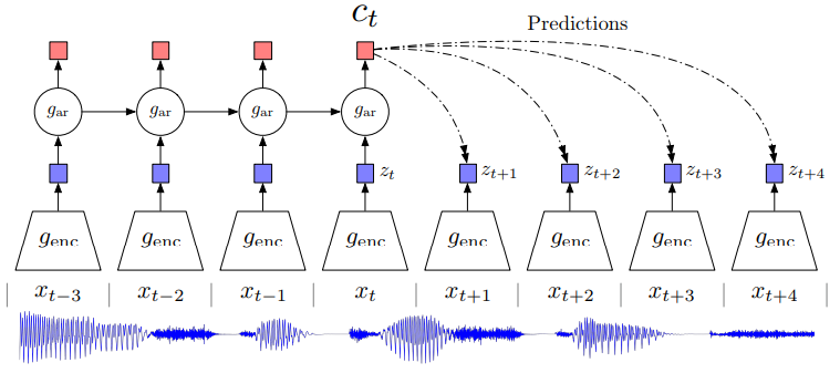
Overview of Contrastive Predictive Coding, the proposed representation learning approach. Although this figure shows audio as input, we use the same setup for images, text and reinforcement learning.

• Universal unsupervised learning approach to extract useful representations from high-dimensional data, called Contrastive Predictive Coding
• Encode the underlying shared information between different parts of the (high-dimensional) signal, discard low-level information and noise that is more local
• Learn representations by predicting the future in latent space by using autoregressive models
  • First, an encoder maps the input sequence \(x_t\) to latent representations \(z_t\) with a lower temporal resolution, next an autoregressive model summarizes multiple latent representations \(z_{\leq t}\) in a context latent representation \(c_t\)
  • Do not predict future observations with a generative model \(p(x_{t+k} \rvert c_{t})\) but model a density ratio which preserves the mutual information between \(x_{t+k}\) and \(c_t\): \(\frac{p(x_{t+k} \rvert c_{t})}{p(x_{t+k}}\)

One of the challenges of predicting high-dimensional data is that unimodal losses such as meansquared error and cross-entropy are not very useful, and powerful conditional generative models which need to reconstruct every detail in the data are usually required. But these models are computationally intense, and waste capacity at modeling the complex relationships in the data \(x\), often ignoring the context \(c\). This suggests that modeling \(p(x|c)\) directly may not be optimal for the purpose of extracting shared information between \(x\) and \(c\). When predicting future information we instead encode the target \(x\) (future) and context \(c\) (present) into a compact distributed vector representations

• Also tested for speech recognition
  • Use raw signal, network consists of a CNN feature extractor and GRU RNN for the autoregressive part

Take-Away:

• Predicting "original" data is difficult, it is much easier to predict an embedding vector
• Two steps: Map input into latent space and then apply autoregressive model

Autoregressive Predictive Coding (APC)

Source: Chung et al, "An Unsupervised Autoregressive Model for Speech Representation Learning", 2019 and Chung et al., "Generative Pre-Training for Speech with Autoregressive Predictive Coding", 2020

• Learn features which preserve information for a wide range of downstream tasks (do not remove noise and speaker variability but retain in the representations as much information about the original signal as possible)
  • Let the downstream task identify which features are helpful and which are not
• Autoregressive Predictive Coding (APC) -> Fed a frame into an RNN to predict one frame in the future
  • Used input: log Mel-Spectrograms
  • L1-Loss
• Note: They solve a different task: The only predict one frame and then only use hidden embeddings for other downstream tasks.

Take-away

• Try MAE instead of MSE as loss
• Try RNN network
  • Even though Transformer were found superior
• Only predict one frame ahead but multiple times (shift window)
  • Further away to learn more global structures instead of exploiting local smoothness
• Use large dataset for pretraining

Learning Speaker Representations with Mutual Information

Source: Ravanelli and Bengio, "Learning Speaker Representations with Mutual Information", 2018

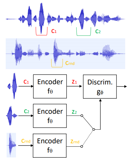
Architecture of the proposed system for unsupervised learning of speaker representations. The speech chunks c_1 and c_2 are sampled from the same sentence, while c_rand is sampled from a different utterance.

• Learn representations that capture speaker identities by maximizing the mutual information between the encoded representations of chunks of speech randomly sampled from the same sentence
  • Mutial information (MI): This measure is a fundamental quantity for estimating the statistical dependence between random variables. As opposed to other metrics, such as correlation, MI can capture complex non-linear relationships between random variables
    • MI is difficult to compute directly. The aforementioned works found that it is possible to maximize or minimize the MI within a framework that closely resembles that of GANs
• Encoder relies on the SincNet architecture and transforms raw speech waveform into a compact feature vector
• Discriminator is fed by either positive samples (of the joint distribution of encoded chunks) or negative samples (from the product of the marginals) and is trained to separate them.
  • Is fed by samples from the joint distribution (i.e. two local encoded vectors randomly drawn from the same speech sentence) and from the product of marginal distributions (i.e, two local encoder vectors coming different utterances). The discriminator is jointly trained with the encoder to maximize the separability of the two distributions.
• positive samples are simply derived by randomly sampling speech chunks from the same sentence. Negative samples, instead, are obtained by randomly sampling from another utterance. The underlying assumptions considered here are the following: (1) two random utterances likely belong to different speakers, (2) each sentence contains a single speaker only.
• Differently to the GAN framework, the encoder and the discriminator are not adversarial here but must cooperate to maximize the discrepancy between the joint and the product of marginal distributions (max-max game instead of min-max game)
• The best results are obtained with end-to-end semi-supervised learning, where an ecosystem of neural networks composed of an encoder, a discriminator, and a speaker-id must cooperate to derive good speaker embeddings

wav2vec: Unsupervised Pre-Training for Speech Recognition

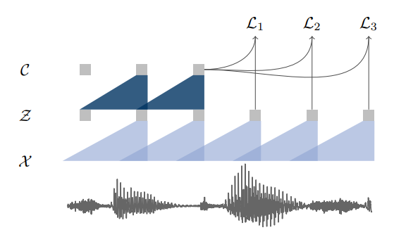
Illustration of pre-training from audio data X which is encoded with two convolutional neural networks that are stacked on top of each other. The model is optimized to solve a next time step prediction task.

• Convolutional neural network optimized via a noise contrastive binary classification task
  • Input: Raw audio
  • Encoder networks embeds the audio signal in a latent space (i.e. convert raw audio to latent representations), context network combines multiple time-steps of the encoder to obtain contextualized representations (i.e. mix multiple latent representations to contextualized tensor with a given receptive field)
    • Important: use skip connections and (group) normalization
  • Contrastive loss that requires distinguishing a true future audio sample from distractor samples
• Mainly used for speech to text conversion: Therefore a lexicon as well as a seperate language model was used after a beam search decoder
• Uses the same loss function as word2vec

Given an audio signal as input, we optimize our model to predict future samples from a given signal context. A common problem with these approaches is the requirement to accurately model the data distribution \(p(x)\), which is challenging. We avoid this problem by first encoding raw speech samples x into a feature representation z at a lower temporal frequency and then implicitly model a density ratio \(p(z_{i+k}|z_{i} ... z_{i−r})/p(z_{i+k})\) similar to [Representation learning with contrastive predictive coding]

k: number of steps in the future

wav2vec with Quantization

Source: Baevski et al., "vq-wav2vec: Self-Supervised Learning of Discrete Speech Representations". 2019 and Source: Baevski and Mohamed, "Effectiveness of Self-Supervised Pre-Training for ASR", 2020, ICASSP

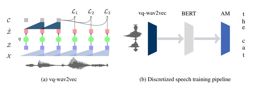
(a) The vq-wav2vec encoder maps raw audio (X) to a dense representation (Z) which is quantized (q) to Zˆ and aggregated into context representations (C); training requires future time step prediction. (b) Acoustic models are trained by quantizing the raw audio with vq-wav2vec, then applying BERT to the discretized sequence and feeding the resulting representations into the acoustic model to output transcriptions.

• Combine the two methods wav2veq and BERT to transform audio to text
• vq-wav2vec uses an additional quantization module (a CNN to build discrete representations) after calculating the dense representations and before aggregating them to context representations
  • More accurate with quantization module
• Fine-tune the pre-trained BERT models on transcribed speech using a Connectionist Temporal Classification (CTC) loss instead of feeding the representations into a task-specific model

wav2vec 2.0: A Framework for Self-Supervised Learning of Speech Representations

Source: Baevski et al., "wav2vec 2.0: A Framework for Self-Supervised Learning of Speech Representations", 2020

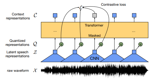
Illustration of the framework which jointly learns contextualized speech representations and an inventory of discretized speech units.

• wav2vec 2.0 masks the speech input in the latent space and solves a contrastive task defined over a quantization of the latent representations which are jointly learned.
  • Input raw audio data in encoder (CNN) and then masks spans of the resulting latent speech representations. The latent representations are fed to a Transformer network to build contextualized representations and the model is trained via a contrastive task where the true latent is to be distinguished from distractors
  • Main difference to vq-wav2vec: Train End-to-End with one network

Speech Synthesis

Source: Wang et al., "Tacotron: Towards End-to-End Speech Synthesis", 2017 and Chung et al., "Semi-Supervised Training for Improving Data Efficiency in End-to-End Speech Synthesis", ICASSP, 2019

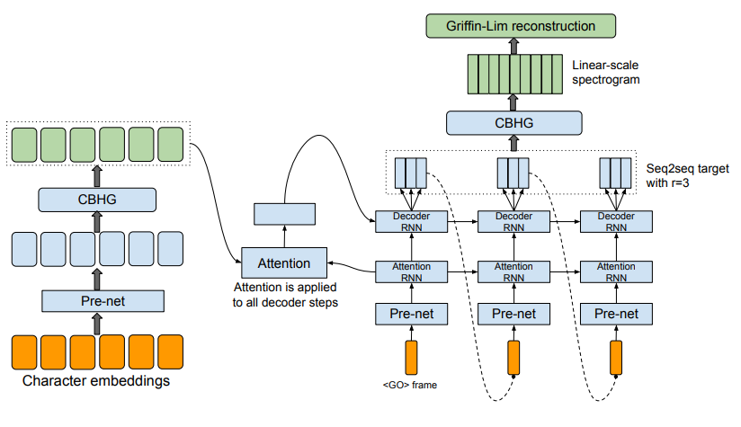
Tactron model architecture. The model takes characters as input and outputs the corresponding raw spectrogram, which is then fed to the Griffin-Lim reconstruction algorithm to synthesize speech.

• Tacotron: Takes characters as input and outputs raw spectrogram frames, which are then converted to waveforms
  • The backbone of Tacotron is a modified seq2seq model with attention. The model consists of an encoder, an attention-based decoder, and a post-processing net.
  • The goal of the encoder is to extract robust sequential representations of text.
• Both approaches used L1-Loss